Interpolation types

NAVIGATION: Motion profile > Interpolation types

Interpolation types

General definition of interpolation

If only individual points of a function are known, but no analytical description of the function in order to evaluate it at random locations, a suitable interpolation method is applied to estimate the function at the points in-between. This is termed an interpolation problem. There are a number of solutions to the problem; the user must select the appropriate functions. Depending on the functions chosen, a different interpolant is obtained.
Interpolation is a kind of approximation: The function under analysis is precisely reproduced by the interpolation function at the interpolation points and at the remaining points is at least approximated. The quality of approximation depends on the method chosen. In order to estimate it, additional information above the function is required. Even if f is not known, this is usually obtained naturally: The limitation, consistency or differentiation capacity can frequently be assumed.

Linear interpolation	Function
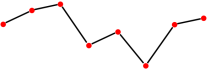
	Linear interpolation: Here two given datum points f₀ and f₁ are connected by a line. To n+1 differing datum point pairs there is exactly one n-th order interpolation polynomial, which matches at the specified interpolation points.

Linear interpolation

Function

Linear interpolation:

Here two given datum points
f₀ and f₁ are connected by a line.

To n+1 differing datum point pairs there is exactly one n-th order interpolation polynomial, which matches at the specified interpolation points.

Bild: Linear interpolation

Cubic interpolation	Function
	As polynomials become more and more unstable as the order of magnitude increases – that is to say, fluctuate widely between the interpolation points – in practice polynomials of an order greater than 5 are rarely applied. Instead, large data sets are interpolated in chunks. In the case of linear interpolation, that would be a frequency polygon; in the case of 2nd or 3rd order polynomials the usual term used is spline interpolation. In the case of sectionally defined interpolants, the question of consistency and differentiation at the interpolation points is of major importance.

Cubic interpolation

Function

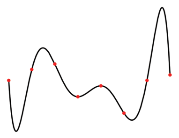
As polynomials become more and more unstable as the order of magnitude increases – that is to say, fluctuate widely between the interpolation points – in practice polynomials of an order greater than 5 are rarely applied. Instead, large data sets are interpolated in chunks. In the case of linear interpolation, that would be a frequency polygon; in the case of 2nd or 3rd order polynomials the usual term used is spline interpolation. In the case of sectionally defined interpolants, the question of consistency and differentiation at the interpolation points is of major importance.

Bild: Cubic interpolation

The following interpolation types are available to select in the controller.

Parameter No.	Parameter Name	Function
P 0370	CON_IP	Interpolation type in IP mode
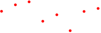
(0)	NoIp(0)	No interpolation: The values are transferred 1:1 to reference processing in 1 ms cycles.
(1)	Lin (1)	Linear interpolation: In the linear interpolation method the acceleration between two points is generally zero. Pre-control of the acceleration values is thus not possible and speed jumps are always caused.
(2)	Spline_Ext_FF(2)	Interpolation with external pre-control: The expected result should exhibit a high degree of contour accuracy and little reference/actual value variation. For more information refer to the bus documentation.
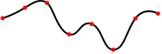
(3)	Splinell(3)	Spline interpolation: In this method interpolation is effected between the interpolation points of the control by means of cubic splines. The trajectory is guided precisely by the control based on the specified points. This may cause a slight jerk at those points, noticeable in the form of "noise". Application: High contouring accuracy, slight "noise" is possible. "Noise" refers to mathematical anomalies which cannot be entirely eliminated by the computing methods applied.
(4)	NonIPSpline(4)	Cubic spline approximation method: In this method the interpolation points are approximated by means of B-splines. The trajectory normally does not run exactly through the points specified by the control. The deviation is normally negligibly small. In the interpolation points the transitions are continuous with regard to acceleration, which becomes apparent by minor "noise". In start and target position the interpolation points always match the trajectory. Application: Minimizing noise, smoother motion, restrictions on contouring
(5)	Cos(5)	Trigonometric interpolation: The interpolation formula corresponds to a Fourier trend of the unknown interpolants.

Tabelle: Interpolation types